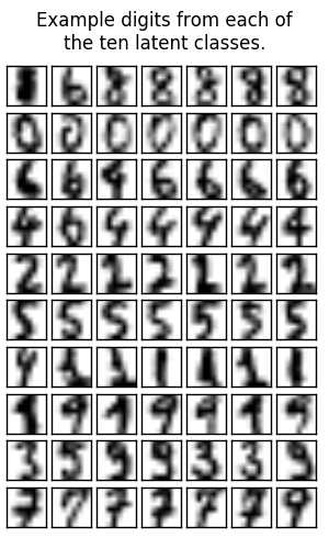
Latent SVM for odd vs. even digit classification¶

A Latent CRF with one node is the same as a latent multiclass SVM Using the latent variables, we can learn non-linear models. This is the same as a simple Latent SVM model. It would obviously be more effiencent to implement a special case for Latent SVMs so we don’t have to run an inference procedure.

This example uses the scikit-learn digit classification dataset, but poses the problem as a binary one, discriminating between even and odd digits.

../_images/sphx_glr_plot_latent_svm_as_crf_001.png

Script output:

Score with binary SVM:
Train: 0.94
Test: 0.91
Score with latent SVM:
Train: 1.00
Test: 0.99
Latent class counts: array([117, 107,  57,  93,  78,  69,  83,  29, 177,  89])

import numpy as np
import matplotlib.pyplot as plt

from sklearn.cross_validation import train_test_split
from sklearn.datasets import load_digits

from pystruct.models import GraphCRF, LatentGraphCRF
from pystruct.learners import NSlackSSVM, LatentSSVM

# Load the scikit-learn digits classification dataset.
digits = load_digits()
X, y_org = digits.data, digits.target
X /= X.max()

# Make binary task by doing odd vs even numers.
y = y_org % 2

# Make each example into a tuple of a single feature vector and an empty edge
# list
X_ = [(np.atleast_2d(x), np.empty((0, 2), dtype=np.int)) for x in X]
Y = y.reshape(-1, 1)

X_train_, X_test_, X_train, X_test, y_train, y_test, y_org_train, y_org_test =\
    train_test_split(X_, X, Y, y_org, test_size=.5)

# First, perform the equivalent of the usual SVM.  This is represented as
# a CRF problem with no edges.

pbl = GraphCRF(inference_method='unary')
# We use batch_size=-1 as a binary problem can be solved in one go.
svm = NSlackSSVM(pbl, C=1, batch_size=-1)

svm.fit(X_train_, y_train)

# Now, use a latent-variabile CRF model with SVM training.
# 5 states per label is enough capacity to encode the 5 digit classes.

latent_pbl = LatentGraphCRF(n_states_per_label=5,
                            inference_method='unary')
base_ssvm = NSlackSSVM(latent_pbl, C=1, tol=.01,
                       inactive_threshold=1e-3, batch_size=10)
latent_svm = LatentSSVM(base_ssvm=base_ssvm, latent_iter=2)
latent_svm.fit(X_train_, y_train)

print("Score with binary SVM:")
print("Train: {:2.2f}".format(svm.score(X_train_, y_train)))
print("Test: {:2.2f}".format(svm.score(X_test_, y_test)))

print("Score with latent SVM:")
print("Train: {:2.2f}".format(latent_svm.score(X_train_, y_train)))
print("Test: {:2.2f}".format(latent_svm.score(X_test_, y_test)))

h_pred = np.hstack(latent_svm.predict_latent(X_test_))
print("Latent class counts: %s" % repr(np.bincount(h_pred)))

# plot first few digits from each latent class

plt.figure(figsize=(3, 5))
plt.suptitle("Example digits from each of\nthe ten latent classes.")
n_latent_classes = 10
n_examples = 7
for latent_class in range(n_latent_classes):
    examples = X_test[h_pred == latent_class][:n_examples]
    for k, example in enumerate(examples):
        plt.subplot(n_latent_classes, n_examples,
                    1 + (n_examples * latent_class + k))
        plt.imshow(example.reshape((8, 8)), cmap=plt.cm.gray_r)
        plt.xticks(())
        plt.yticks(())
plt.subplots_adjust(.02, .04, .96, .88, .12, .18)
plt.show()

Total running time of the script: (0 minutes 15.597 seconds)

Download Python source code: plot_latent_svm_as_crf.py