Details on model specification¶

For those interested in what happens behind the scenes, or those who might want to adjust a model, there is a short explanation of these functions for each model below. For all models, the joint_feature(x, y) function takes a data point and a tentative prediction, and computes a continuous vector of a fixed length that captures the relation between features and label. Learning (that is learner.fit(X, y)) will learn a parameter vector w, and predictions will be made using

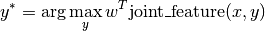
That means the number of parameters in the model is the same as the dimensionality of joint_feature.

The actual maximization is performed in the inference(x, w) function, which takes a sample x and a parameter vector w and outputs a y^*, which (at least approximately) maximizes the above equation.

The loss(y_true, y_pred) function gives a numeric loss for a ground truth labeling y_true and a prediction y_pred, and finally loss_augmented_inference(x, y, w) gives an (approximate) maximizer for

A good place to understand these definitions is Multi-class SVM.

Details on the implementation¶

For this simple model, the joint_feature(x, y) is a vector of size n_features * n_classes, which corresponds to one copy of the input features for each possibly class. For any given pair (x, y) the features in x will be put at the position corresponding to the class in y. Correspondingly, the weights that are learned are one vector of length n_features for each class: w = np.hstack([w_class_0, ..., w_class_1]).

For this simple model, and inference is just the argmax over the inner product with each of these w_class_i:

>>> y_pred = np.argmax(np.dot(w.reshape(n_classes, n_features), x)) 

To perform max-margin learning, we also need the loss-augmented inference. PyStruct has an optimized version, but a pure python version would look like this:

>>> scores = np.dot(w.reshape(n_classes, n_features), x) 
>>> scores[np.arange(n_classes) != y] += 1               
>>> y_pred = np.argmax(scores)                           

Essentialy the response (score / energy) of wrong label is down weighted by 1, the loss of doing an incorrect prediction.

Details on the implementation¶

The model creates a graph over n_classes binary nodes, together with edges between each pair of classes. Each binary node has represents one class, and therefor will get its own column in the weight-vector, similar to the crammer-singer multi-class classification.

In addition, there is a pairwise weight between each pair of labels. This leads to a feature function of this form:

The implementation of the inference for this model creates a graph with unary potentials (given by the inner product of features and weights), and pairwise potentials given by the pairwise weight. This graph is then passed to the general graph-inference, which runs the selected algorithm.

ChainCRF¶

One of the most common use-cases for structured prediction is chain-structured outputs, implemented in models.ChainCRF. These occur naturaly in sequence labeling tasks, such as Part-of-Speech tagging or named entity recognition in natural language processing, or segmentation and phoneme recognition in speech processing.

As an example dataset, we will use the toy OCR dataset letters. In this dataset, each sample is a handwritten word, segmented into letters. This dataset has a slight oddity, in that the first letter of every word was removed, as it was capitalized, and therefore different from all the other letters.

Each letter is a node in our chain, and neighboring letters are connected with an edge. The length of the chain varies with the number of letters in the word. As in all CRF-like models, the nodes in models.ChainCRF all have the same meaning and share parameters.

The letters dataset comes with prespecified folds, we take one fold to be the training set, and the rest to be the test set, as in Max-Margin Markov Networks:

>>> from pystruct.datasets import load_letters
>>> letters = load_letters()
>>> X, y, folds = letters['data'], letters['labels'], letters['folds']
>>> X, y = np.array(X), np.array(y)
>>> X_train, X_test = X[folds == 1], X[folds != 1]
>>> y_train, y_test = y[folds == 1], y[folds != 1]
>>> len(X_train)
704
>>> len(X_test)
6173

The training data is a array of samples, where each sample is a numpy array of shape (n_nodes, n_features). Here n_nodes is the length of the input sequence, that is the length of the word in our case. That means the input array actually has dtype object. We can not store the features in a simple array, as the input sequences can have different length:

>>> X_train[0].shape
(9, 128)
>>> y_train[0].shape
(9,)
>>> X_train[10].shape
(7, 128)
>>> y_train[10].shape
(7,)

Edges don’t need to be specified, as the input features are assumed to be in the order of the nodes in the chain.

The default inference method is max-product message passing on the chain (aka viterbi), which is always exact and efficientl. We use the learners.FrankWolfeSSVM, which is a very efficient learner when inference is fast:

>>> from pystruct.models import ChainCRF
>>> from pystruct.learners import FrankWolfeSSVM
>>> model = ChainCRF()
>>> ssvm = FrankWolfeSSVM(model=model, C=.1, max_iter=10)
>>> ssvm.fit(X_train, y_train) 
FrankWolfeSSVM(C=0.1, batch_mode=False, check_dual_every=10,
            do_averaging=True, line_search=True, logger=None, max_iter=10,
            model=ChainCRF(n_states: 26, inference_method: max-product),
            n_jobs=1, random_state=None, sample_method='perm',
            show_loss_every=0, tol=0.001, verbose=0)
>>> ssvm.score(X_test, y_test) 
0.78...

Details on the implementation¶

The unary potentials in each node are given as the inner product of the features at this node (the input image) with the weights (which are shared over all nodes):

The pairwise potentials are identical over the whole chain and given simply by the weights:

In principle it is possible to also use feature in the pairwise potentials. This is not implemented in the models.ChainCRF, but can be done using EdgeFeatureGraphCRF.

GraphCRF¶

The models.GraphCRF model is a generalization of the ChainCRF to arbitray graphs. While in the chain model, the direction of the edge is usually important, for many graphs, the direction of the edge has no semantic meaning. Therefore, by default, the pairwise interaction matrix of the models.GraphCRF is forced to be symmetric.

Each training sample for the models.GraphCRF is a tuple (features, edges), where features is a numpy array of node-features (of shape (n_nodes, n_features)), and edges is a array of edges between nodes, of shape (n_edges, 2). Each row of the edge array are the indices of the two nodes connected by the edge, starting from zero.

To reproduce the models.ChainCRF model above with models.GraphCRF, we can simply generate the indices of a chain:

>>> features, y, folds = letters['data'], letters['labels'], letters['folds']
>>> features, y = np.array(features), np.array(y)
>>> features_train, features_test = features[folds == 1], features[folds != 1]
>>> y_train, y_test = y[folds == 1], y[folds != 1]

For a single word made out of 9 characters:

>>> features_0 = features_train[0]
>>> features_0.shape
(9, 128)
>>> n_nodes = features_0.shape[0]
>>> edges_0 = np.vstack([np.arange(n_nodes - 1), np.arange(1, n_nodes)])
>>> edges_0
array([[0, 1, 2, 3, 4, 5, 6, 7],
       [1, 2, 3, 4, 5, 6, 7, 8]])
>>> x = (features_0, edges_0)

For the whole training dataset:

>>> f_t = features_train
>>> X_train = [(features_i, np.vstack([np.arange(features_i.shape[0] - 1), np.arange(1, features_i.shape[0])]))
...            for features_i in f_t]
>>> X_train[0] 
(array([[0, 0, 0, ..., 0, 0, 0],
   [0, 0, 0, ..., 0, 0, 0],
   [0, 0, 0, ..., 0, 0, 0],
   ...,
   [0, 0, 0, ..., 0, 0, 0],
   [0, 0, 0, ..., 0, 0, 0],
   [0, 0, 1, ..., 0, 1, 1]], dtype=uint8), array([[0, 1, 2, 3, 4, 5, 6, 7],
   [1, 2, 3, 4, 5, 6, 7, 8]]))

Now we can fit a (directed) models.GraphCRF on this data:

>>> from pystruct.models import GraphCRF
>>> from pystruct.learners import FrankWolfeSSVM
>>> model = GraphCRF(directed=True, inference_method="max-product")
>>> ssvm = FrankWolfeSSVM(model=model, C=.1, max_iter=10)
>>> ssvm.fit(X_train, y_train) 
FrankWolfeSSVM(C=0.1, batch_mode=False, check_dual_every=10,
            do_averaging=True, line_search=True, logger=None, max_iter=10,
            model=GraphCRF(n_states: 26, inference_method: max-product),
            n_jobs=1, random_state=None, sample_method='perm',
            show_loss_every=0, tol=0.001, verbose=0)

Details on the implementation¶

The potentials are the same as in the ChainCRF model, with unary potentials given as a shared linear function of the features, and pairwise potentials the same for all nodes.

EdgeFeatureGraphCRF¶

This model is the most general of the CRF models, and contains all other CRF models as a special case. This model assumes again that the parameters of the potentials are shared over all nodes and over all edges, but the pairwise potentials are now also computed as a linear function of the features.

Each training sample for models.EdgeFeatureGraphCRF is a tuple (node_features, edges, edge_features), where node_features is a numpy array of node-features (of shape (n_nodes, n_node_features)), edges is a array of edges between nodes, of shape (n_edges, 2) as in GraphCRF, and edge_features is a feature for each edge, given as a numpy array of shape (n_edges, n_edge_features).

The edge features allow the pairwise interactions to be modulated by the context. Two features important for image segmentation, for example, are color differences between the (super)pixels at given nodes, and whether one is above the other. If two neighboring nodes correspond to regions of simlar color, they are more likely to have the same label. For the vertical direction, a node above a node representing “sky” is more likely to also represent “sky” than “water”.

A great example of the importance of edge features is Conditional Interactions on the Snakes Dataset.

LatentGraphCRF aka Hidden Dynamics CRF¶

models.LatentGraphCRF implements the “Hidden Dynamics CRF” approach. Here, each output state is split into several hidden sub-states, which allows for more complex interactions.

This can be seen as a structured variant of the latent SVM approach as follows: If there is a single node in the graph (that is doing multi-class classification), we introduce latent subclasses for each of the target classes. We can then learn a separate classifier for each of the subclasses, which might be easier. An example is given in Latent SVM for odd vs. even digit classification, where images of odd numbers are classified against images of even numbers. It is much easier to learn a linear classifier that separates one digit from the other digits, than trying to learn a linear separation between even and odd digits.

For more complex graphs, not only the unary potentials benefit, but also the pairwise potentials, which are now between substates. The original paper motivates this extension by action recognition. A complex action like a juming jack is made up of several distinct sub-actions, and there is a distinct order in which the sub-actions are performed. The latent dynamic CRF can learn this order.

See Latent Dynamics CRF for an example on a 2d grid.